1. Introduction
1.1. Overview
The Community Data Management System is an object-oriented data management system, specialized for organizing multidimensional, gridded data used in climate analysis and simulation.
CDMS is implemented as part of the Climate Data Analysis Tool [CDAT](https://cdat.llnl.gov/), which uses the Python language. The examples in this chapter assume some familiarity with the language and the Python Numpy module (http://www.numpy.org). A number of excellent tutorials on Python are available in books or on the Internet. For example, see the Python Foundation’s homepage.
1.2. Variables
The basic unit of computation in CDMS is the variable. A variable is essentially a multidimensional data array,
augmented with a domain, a set of attributes, and optionally a spatial and/or temporal coordinate system
(see Coordinate Axes). As a data array, a variable can be sliced to obtain a portion of the
data, and can be used in arithmetic computations. For example, if u and v are variables representing
the eastward and northward components of wind speed, respectively, and both variables are functions of time,
latitude, and longitude, then the velocity for time 0 (first index) can be calculated as:
>>> # wget "http://cdat.llnl.gov/cdat/sample_data/clt.nc"
>>> f1=cdms2.open("clt.nc")
>>> u = f1('u')
>>> v = f1('v')
>>> from cdms2 import MV2
>>> vel = MV2.sqrt(u[0]**2 + v[0]**2)
This illustrates several points:
Square brackets represent the slice operator. Indexing starts at 0, so
u[0]selects from variableufor the first timepoint. The result of this slice operation is another variable. The slice operator can be multidimensional, and follows the syntax of Numpy Python arrays. In this example,u[0:10,:,1]would retrieve data for the first ten timepoints, at all latitudes, for the second longitude.Variables can be used in computation.
**is the Python exponentiation operator.Arithmetic functions are defined in the
cdms2.MV2module.Operations on variables carry along the corresponding metadata where applicable. In the above example,
velhas the same latitude and longitude coordinates asuandv, and the time coordinate is the first time ofuandv.
1.3. File I/O
A variable can be obtained from a file or collection of files, or can be generated as the result of a computation.
Files can be in any of theself- describing formats:
netCDF, HDF, GrADS/GRIB (GRIB with a GrADS control file), or PCMDI DRS.
Note: (HDF and DRS support is optional, and is configured at the time CDAT is installed.)
For instance, to read datafrom file sample.nc into variable u:
>>> # wget "http://cdat.llnl.gov/cdat/sample_data/clt.nc"
>>> f = cdms2.open('clt.nc')
>>> u = f('u')
Data can be read by index or by world coordinate values. The following reads the n-th timepoint of u (the syntax slice(i,j) refers to indices k such that i <= k < j):
>>> n = 0
>>> u0 = f('u',time=slice(n,n+1))
To read u at time 1.:
>>> u1 = f('u',time=1.)
A variable can be written to a file with the write function:
>>> g = cdms2.open('sample2.nc','w')
>>> g.write(u)
<cdms2.fvariable.FileVariable object at ...
>>> g.close()
1.4. Coordinate Axes
A coordinate axis is a variable that represents coordinate information. Typically an axis is associated with one or more variables in a file or dataset, to represent the indexing and/or spatiotemporal coordinate system(s) of the variable(s).
Often in climate applications an axis is a one-dimensional variable whose values are floating-point and strictly monotonic. In some cases an axis can be multidimensional (see Grids). If an axis is associated with one of the canonical types latitude, longitude, level, or time, then the axis is called temporal .
The shape and physical ordering of a variable is represented by the
variables domain , an ordered tuple of one-dimensional axes. In the
previous example, the domain of the variable u is the tuple (time,
latitude, longitude). This indicates the order of the dimensions, with
the slowest-varying dimension listed first (time). The domain may be
accessed with the getAxisList() method:
>>> u.getAxisList()
[   id: time1
Designated a time axis.
units:  months since 1978-12
Length: 1
First:  1.0
Last:   1.0
Other axis attributes:
   calendar: gregorian
   axis: T
Python id:  ...
,    id: plev
Designated a level axis.
units:  hPa
Length: 2
First:  200.0
Last:   850.0
Other axis attributes:
   axis: Z
   realtopology: linear
Python id:  ...
,    id: latitude1
Designated a latitude axis.
units:  degrees_north
Length: 80
First:  -88.2884
Last:   88.2884
Other axis attributes:
   axis: Y
   realtopology: linear
Python id:  ...
,    id: longitude1
Designated a longitude axis.
units:  degrees_east
Length: 97
First:  -180.0
Last:   180.0
Other axis attributes:
   axis: X
   topology: circular
   modulo: 360.0
   realtopology: linear
Python id:  ...
]
In the above example, the domain elements are axes that are also spatiotemporal. In general it is not always the case that an element of a domain is spatiotemporal:
An axis in the domain of a variable need not be spatiotemporal. For example, it may represent a range of indices, an index coordinate system.
The latitude and/or longitude coordinate axes associated with a variable need not be elements of the domain. In particular this will be true if the variable is defined on a non-rectangular grid (see Grids).
As previously noted, a spatial and/or temporal coordinate system may be associated with a variable. The methods getLatitude, getLongitude, getLevel, and getTime return the associated coordinate axes. For example:
>>> t = u.getTime()
>>> print t[:]
[ 1.]
>>> print t.units
months since 1978-12
1.5. Attributes
As mentioned above, variables can have associated attributes , name-value pairs. In fact, nearly all CDMS objects can have associated attributes, which are accessed using the Python dot notation:
>>> u.units='m/s'
>>> print u.units
m/s
Attribute values can be strings, scalars, or 1-D Numpy arrays.
When a variable is written to a file, not all the attributes are written. Some attributes, called internal attributes, are used for bookkeeping, and are not intended to be part of the external file representation of the variable. In contrast, external attributes are written to an output file along with the variable. By default, when an attribute is set, it is treated as external. Every variable has a field attributes, a Python dictionary that defines the external attributes:
>>> print u.attributes.keys()
'name', 'title', 'tileIndex', 'date', 'source', 'time', 'units', 'type']
The Python dir command lists the internal attribute names:
>>> dir(u)
['T', '_FillValue', '_TransientVariable__domain', ..., 'view']
In general internal attributes should not be modified directly. One exception is the id attribute, the name of the variable. It is used in plotting and I/O, and can be set directly.
1.6. Masked Values
Optionally, variables have a mask that represents where data are missing. If present, the mask is an array of ones and zeros having the shape of the data array. A mask value of one indicates that the corresponding data array element is missing or invalid.
Arithmetic operations in CDMS take missing data into account. The same is true of the functions defined in the cdms2.MV2 module. For example:
>>> a = MV2.array([1,2,3]) # Create array a, with no mask
>>> b = MV2.array([4,5,6]) # Same for b
>>> a+b # variable_... array([5,7,9,])
variable_...
masked_array(data = [5 7 9],
         mask = False,
    fill_value = 999999)
>>>
>>>
>>> a[1]=MV2.masked # Mask the second value of a a.mask()
>>> a.mask
array([False,  True, False], dtype=bool)
>>> a+b # The sum is masked also
variable_...
masked_array(data = [5 -- 9],
         mask = [False  True False],
    fill_value = 999999)
When data is read from a file, the result variable is masked if the file variable has a missing_value attribute. The mask is set to one for those elements equal to the missing value, zero elsewhere. If no such attribute is present in the file, the result variable is not masked.
When a variable with masked values is written to a file, data values
with a corresponding mask value of one are set to the value of the
variables missing_value attribute. The data and missing_value
attribute are then written to the file.
Masking is covered in Section 2.9. See also the
documentation of the Python Numpy and MA modules, on which cdms2.MV2
is based, at
1.7. File Variables
A variable can be obtained either from a file, a collection of files, or as the result of computation. Correspondingly there are three types of variables in CDMS:
file variable is a variable associated with a single data file. Setting or referencing a file variable generates I/O operations.
dataset variable is a variable associated with a collection of files. Reference to a dataset variable reads data, possibly from multiple files. Dataset variables are read-only.
transient variable is an in-memory object not associated with a file or dataset. Transient variables result from a computation or I/O operation.
Typical use of a file variables is to inquire information about the
variable in a file without actually reading the data for the variables.
A file variable is obtained by applying the slice operator [] to a file,
passing the name of the variable, or by calling the getVariable
function.
Note That obtaining a file variable does not actually read the data array:
>>> u = f.getVariable('u') # or u=f['u']
>>> u.shape
(1, 2, 80, 97)
File variables are also useful for fine-grained I/O. They behave like transient variables, but operations on them also affect the associated file. Specifically:
slicing a file variable reads data,
setting a slice writes data,
referencing an attribute reads the attribute,
setting an attribute writes the attribute,
and calling a file variable like a function reads data associated with the variable:
>>> import os
>>> os.system("cp clt.nc /tmp")
0
>>> f = cdms2.open('/tmp/clt.nc','a') # Open read/write
>>> uvar = f['u'] # Note square brackets
>>> uvar.shape
(1, 2, 80, 97)
>>> u0 = uvar[0] # Reads data from sample.nc
>>> u0.shape
(2, 80, 97)
>>> uvar[1]=u0 # Writes data to sample.nc
>>> uvar.units # Reads the attribute 'm/s'
'm/s'
>>> u24 = uvar(time=1.0) # Calling  a variable like a function reads data
>>> f.close() # Save changes to clt.nc (I/O may be buffered)
For transient variables, the data is printed only if the size of the array is less than the print limit . This value can be set with the function MV2.set_print_limit to force the data to be printed:
>>> MV2.get_print_limit() # Current limit 1000
1000
>>> smallvar
small variable
masked_array(data =
  [[  0.   1.   2.   3.   4.]
  [  5.   6.   7.   8.   9.]
  [ 10.  11.  12.  13.  14.]
  [ 15.  16.  17.  18.  19.]],
   mask =
  False,
        fill_value = 999999.0)
>>> MV2.set_print_limit(100)
>>> largevar
large variable
masked_array(data =
[[   0.    1.    2. ...,   17.   18.   19.]
[  20.   21.   22. ...,   37.   38.   39.]
[  40.   41.   42. ...,   57.   58.   59.]
...,
[ 340.  341.  342. ...,  357.  358.  359.]
[ 360.  361.  362. ...,  377.  378.  379.]
[ 380.  381.  382. ...,  397.  398.  399.]],
mask = False,
fill_value = 999999.0)
The datatype of the variable is determined with the typecode function:
>>> u.typecode()
'f'
1.8. Dataset Variables
The third type of variable, a dataset variable, is associated with a
dataset, a collection of files that is treated as a single file. A
dataset is created with the cdscan utility. This generates an XML
metafile that describes how the files are organized and what metadata
are contained in the files. In a climate simulation application, a
dataset typically represents the data generated by one run of a general
circulation or coupled ocean-atmosphere model.
For example, suppose data for variables u and v are stored in six files:
u_2000.nc,
u_2001.nc,
u_2002.nc,
v_2000.nc,
v_2001.nc,
v_2002.nc.
A metafile can be generated with the command:
$ cdscan -x cdsample.xml [uv]*.nc
The metafile cdsample.xml is then used like an ordinary data file:
>>> import os
>>> os.system("cdscan -x cdsample.xml [uv]*.nc")
0
>>> f = cdms2.open('cdsample.xml')
>>> u = f('u')
>>> u.shape
(3, 16, 32)
1.9. Grids
A latitude-longitude grid represents the coordinate information associated with a variable. A grid encapsulates:
latitude, longitude coordinates
grid cell boundaries
area weights
CDMS defines a rich set of grid types to represent the variety of coordinate systems used in climate model applications. Grids can be categorized as rectangular or nonrectangular.
A rectangular grid has latitude and longitude axes that are one-dimensional, with strictly monotonic values. The grid is essentially the Cartesian product of the axes. If either criterion is not met, the grid is nonrectangular .
CDMS supports two types of nonrectangular grid:
A curvilinear grid consists of a latitude and longitude axis, each of which is a two-dimensional coordinate axis. Curvilinear grids are often used in ocean model applications.
A generic grid consists of a latitude and longitude axis, each of which is an auxiliary one-dimensional coordinate axis. An auxiliary axis has values that are not necessarily monotonic. As the name suggests, generic grids can represent virtually any type of grid. However, it is more difficult to determine adjacency relationships between grid points.
1.9.1. Example: A Curvilinear Grid
In this example, variable sample is defined on a 128x192 curvilinear grid. Note that:
The domain of variable sample is ( y , x ) where y and x are index coordinate axes.
The curvilinear grid associated with sample consists of axes ( lat , lon ), each a two-dimensional coordinate axis.
lat and lon each have domain ( y , x )
>>> f = cdms2.open('sampleCurveGrid4.nc')
>>> # lat and lon are coordinate axes, but are grouped with data variables
>>> f.variables.keys()
['lat', 'sample', 'bounds_lon', 'lon', 'bounds_lat']
>>> # y and x are index coordinate axes
>>> f.axes.keys()
['nvert', 'x', 'y']
>>> # Read data for variable sample
>>> sample = f('sample')
>>> # The associated grid g is curvilinear
>>> g = sample.getGrid()
>>> # The domain of the variable consists of index axes
>>> sample.getAxisIds()
['y', 'x']
>>> # Get the coordinate axes associated with the grid
>>> lat = g.getLatitude() # or sample.getLatitude()
>>> lon = g.getLongitude() # or sample.getLongitude()
>>> # lat and lon have the same domain, a subset of the domain of 'sample'
>>> lat.getAxisIds()
['y', 'x']
>>> # lat and lon are variables ...
>>> lat.shape
(32, 48)
>>> lat
lat
masked_array(data =
[[-76.08465554 -76.08465554 -76.08465554 ..., -76.08465554 -76.08465554
-76.08465554]
[-73.92641847 -73.92641847 -73.92641847 ..., -73.92641847 -73.92641847
-73.92641847]
[-71.44420823 -71.44420823 -71.44420823 ..., -71.44420823 -71.44420823
-71.44420823]
...,
[ 42.32854943  42.6582209   43.31990211 ...,  43.3199019   42.65822088
42.32854943]
[ 42.70106429  43.05731498  43.76927818 ...,  43.76927796  43.05731495
42.70106429]
[ 43.0307341   43.41264383  44.17234165 ...,  44.17234141  43.41264379
43.0307341 ]],
mask = False, fill_value = 1e+20)
>>> lat_in_radians = lat*MV2.pi/180.0
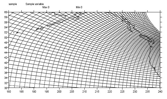
Figure 1: Curvilinear Grid
1.9.2. Example: A Generic Grid
In this example variable zs is defined on a generic grid. Figure 2 illustrates the grid, in this case a geodesic grid:
>>> f.variables.keys()
['lat', 'sample', 'bounds_lon', 'lon', 'bounds_lat']
>>> f.axes.keys()
['nvert', 'x', 'y']
>>> zs = f('sample')
>>> g = zs.getGrid()
>>> g
<TransientCurveGrid, id: ..., shape: (32, 48)>
>>> lat = g.getLatitude()
>>> lon = g.getLongitude()
>>> lat.shape
(32, 48)
>>> lon.shape # variable zs is defined in terms of a single index coordinate
(32, 48)
>>> # axis, 'cell'
>>> zs.shape
(32, 48)
>>> zs.getAxisIds()
['y', 'x']
>>> # lat and lon are also defined in terms of the cell axis
>>> lat.getAxisIds()
['y', 'x']
>>> # lat and lon are one-dimensional, 'auxiliary' coordinate
>>> # axes: values are not monotonic
>>> lat.__class__
<class 'cdms2.coord.TransientAxis2D'>
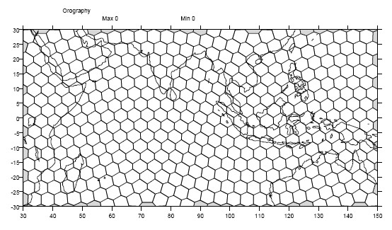
Figure 2: Generic Grid
Generic grids can be used to represent any of the grid types. The method toGenericGrid can be applied to any grid to convert it to a generic representation. Similarly, a rectangular grid can be represented as curvilinear. The method toCurveGrid is used to convert a non-generic grid to curvilinear representation:
>>> f = cdms2.open(cdat_info.get_sampledata_path()+'/clt.nc')
>>> clt = f('clt')
>>> rectgrid = clt.getGrid()
>>> rectgrid.shape
(46, 72)
>>> curvegrid = rectgrid.toCurveGrid()
>>> curvegrid
<TransientCurveGrid, id: ..., shape: (46, 72)>
>>> genericgrid = curvegrid.toGenericGrid()
>>> genericgrid
<TransientGenericGrid, id: ..., shape: (3312,)>
1.10. Regridding
Regridding is the process of mapping variables from one grid to another. CDMS supports two forms of regridding. Which one you use depends on the class of grids being transformed:
To interpolate from one rectangular grid to another, use the built-in CDMS regridder. CDMS also has built-in regridders to interpolate from one set of pressure levels to another, or from one vertical cross-section to another.
To interpolate from any lat-lon grid, rectangular or non-rectangular, use the SCRIP regridder.
1.10.1. CDMS Regridder
The built-in CDMS regridder is used to transform data from one
rectangular grid to another. For example, to regrid variable u (from
a rectangular grid) to a 96x192 rectangular Gaussian grid:
>>> f = cdms2.open('clt.nc')
>>> u = f('u')
>>> u.shape
(1, 2, 80, 97)
>>> t63_grid = cdms2.createGaussianGrid(96)
>>> u63 = u.regrid(t63_grid)
>>> u63.shape
(1, 2, 96, 192)
To regrid a variable uold to the same grid as variable vnew:
>>> f = cdms2.open('clt.nc')
>>> uold = f('u')
>>> unew = f2('uwnd')
>>> uold.shape
(1, 2, 80, 97)
>>> unew.shape
(1, 14, 181, 360)
>>> t63_grid = unew.getGrid() # Obtain the grid for vnew
>>> u63 = uold.regrid(t63_grid)
>>> u63.shape
(1, 2, 181, 360)
1.10.2. SCRIP Regridder
To interpolate between any lat-lon grid types, the SCRIP regridder may be used. The SCRIP package was developed at [Los Alamos National Laboratory] (http://oceans11.lanl.gov/drupal/Models/OtherSoftware). SCRIP is written in Fortran 90, and must be built and installed separately from the CDAT/CDMS installation.
The steps to regrid a variable are:
(External to CDMS)
Obtain or generate the grids, in SCRIP netCDF format.
Run SCRIP to generate a remapping file.
(In CDMS)
Read the regridder from the SCRIP remapping file.
Call the regridder with the source data, returning data on the target grid.
Steps 1 and 2 need only be done once. The regridder can be used as often as necessary.
For example, suppose the source data on a T42 grid is to be mapped to a POP curvilinear grid. Assume that SCRIP generated a remapping file named rmp_T42_to_POP43_conserv.nc:
>>> # Import regrid package for regridder functions
>>> import regrid2, cdms2

>>> # Get the source variable
>>> f = cdms2.open('sampleT42Grid.nc')
>>> dat = f('src_array')
>>> f.close()

>>> # Read the regridder from the remapper file
>>> remapf = cdms2.open('rmp_T42_to_POP43_conserv.nc')
>>> regridf = regrid2.readRegridder(remapf)
>>> remapf.close()

>>> # Regrid the source variable
>>> popdat = regridf(dat)
Regridding is discussed in Chapter 4.
1.11. Time Types
CDMS provides extensive support for time values in the cdtime module. cdtime also defines a set of calendars, specifying the number of days in a given month.
Two time types are available: relative time and component time . Relative time is time relative to a fixed base time. It consists of:
a
unitsstring, of the form"units since basetime", anda floating-point
value
For example, the time “28.0 days since 1996-1-1” has value= 28.0 , and units=” days since 1996-1-1”. To create a relative time type:
>>> import cdtime
>>> rt = cdtime.reltime(28.0, "days since 1996-1-1")
>>> rt
28.000000 days since 1996-1-1
>>> rt.value
28.0
>>> rt.units
'days since 1996-1-1'
A component time consists of the integer fields year, month, day, hour, minute, and the floating-point field second. For example:
>>> ct = cdtime.comptime(1996,2,28,12,10,30)
>>> ct
1996-2-28 12:10:30.0
>>> ct.year
1996
>>> ct.month
2
The conversion functions tocomp and torel convert between the two representations. For instance, suppose that the time axis of a variable is represented in units ” days since 1979”. To find the coordinate value corresponding to January 1, 1990:
>>> ct = cdtime.comptime(1990,1)
>>> rt = ct.torel("days since 1979")
>>> rt.value
4018.0
Time values can be used to specify intervals of time to read. The syntax time=(c1,c2) specifies that data should be read for times t such that c1<=t<=c2:
>>> fh = cdms2.open(cdat_info.get_sampledata_path() + "/tas_6h.nc")
>>> c1 = cdtime.comptime(1980,1)
>>> c2 = cdtime.comptime(1980,2)
>>> tas = fh['tas']
>>> tas.shape
(484, 45, 72)
>>> x = tas.subRegion(time=(c1,c2))
>>> x.shape
(125, 45, 72)
or string representations can be used:
>>> fh = cdms2.open(cdat_info.get_sampledata_path() + "/tas_6h.nc")
>>> tas = fh['tas']
>>> x = tas.subRegion(time=('1980-1','1980-2'))
Time types are described in Chapter 3.
1.12. Plotting Data
Data read via the CDMS Python interface can be plotted using the vcs module. This module, part of the Climate Data Analysis Tool (CDAT) is documented in the VCS reference manual. The vcs module provides access to the functionality of the VCS visualization program.
To generate a plot:
Initialize a canvas with the
vcs initroutine.Plot the data using the canvas
plotroutine.
For example:
>>> import cdms2, vcs, cdat_info
>>> fh=cdms2.open(cdat_info.get_sampledata_path() + "/tas_cru_1979.nc")
>>> fh['time'][:] # Print the time coordinates
array([ 1476.,  1477.,  1478.,  1479.,  1480.,  1481.,  1482.,  1483.,
        1484.,  1485.,  1486.,  1487.])
>>>
>>> tas = fh('tas', time=1479)
>>> tas.shape
(1, 36, 72)
>>> w = vcs.init() # Initialize a canvas
>>> w.plot(tas) # Generate a plot
<vcs.displayplot.Dp object at...
By default for rectangular grids, a boxfill plot of the lat-lon slice is produced. Since variable precip includes information on time, latitude, and longitude, the continental outlines and time information are also plotted. If the variable were on a non-rectangular grid, the plot would be a meshfill plot.
The plot routine has a number of options for producing different types of plots, such as isofill and x-y plots. See Chapter 5 for details.